Generating multivariate normal samples

Data generation by MASS::mvrnorm() : as dimension increases

Assuming we do a simulation study for a paper: we may want to check estimation performance, prediction performance, or size and power of a testing procedure. Let’s generate \(p=400\) dimensional normal vectors. You may want \(n\) samples per simulation, let say \(100\). Repeat this procedure multiple times, for example, you do \(500\) repetitions for three settings. If each sampling step takes 0.03 seconds (as the simulation result below), entire data generation would take \(0.03\times 500\times 3 = 45\) seconds. If \(p=1600\), it would take \(0.8\times 500\times 3 = 1200\) seconds.

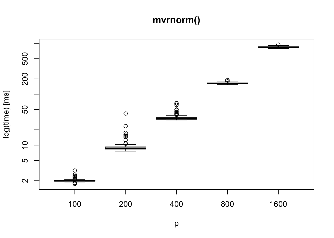
In most of the simulation studies I have done, it would not be a big issue since \(p\) is most likely less than or equal to \(1000\). However, we may need a faster sampling code if we want to use larger \(p\) or consider more simulation settings.

Structure of mvrnorm()

For a mean vector \(\mu\in \mathbb{R}^{p}\) and a covariance matrix \(\Sigma\in \mathbb{R}^{p\times p}\), mvrnorm() generates random samples \(X\in\mathbb{R}^{n\times p}\) from \(N(\mu,\Sigma)\). The structure of the function is the following:

1. Run eigendecomposition on the covariance matrix \(\Sigma = QDQ^{\mathrm{T}}\) where \(D\) is a diagonal matrix of eigenvalues \(d_j, j=1,\ldots p\), and \(Q\) is a matrix whose \(j\)th column is the eigenvector corresponding .
2. Check all the eigenvalues are positive. If some of the eigenvalues are not ``tolerable’, stop the function with an error message.
3. Using the eigenvalues and eigenvectors, computing the scale matrix, \(A=QD^{1/2}\) so that \(\Sigma = A A^{\mathrm{T}}\).
4. Generate a matrix \(Z\in\mathbb{R}^{n\times p}\) whose entries are random samples from \(N(0,1)\).
5. \(X_i = \mu + AZ_i\) where \(X_i\) and \(Z_i\) are \(i\)th row vector of \(X\) and \(Z\), respectively. In matrix form, \(X^{\mathrm{T}} = \mu \times \mathbf{1} + AZ^{\mathrm{T}}\) where \(\mathbf{1}\) is a vector whose entries are 1.

For more details, see Johnson (2016).

##         self.time self.pct total.time total.pct
## "eigen"      0.56    90.32       0.56     90.32
## "%*%"        0.04     6.45       0.04      6.45
## "diag"       0.02     3.23       0.02      3.23

It is worth noting that eigendcomposition is the most computationally expensive part. The profiling result of mvrnorm() above shows that approximately 90% of the computation time is from eigendecompostion where \(n=\) 100, \(p=\) 1000, \(\mu=\mathbf{0}\), and \(\Sigma\) is a banded matrix (specified later).

How to make it faster? For a positive-definite matrix

If we know the matrix is a positive-definite matrix, we don’t need to check whether its eigenvalues are all positive. This implies that we can use faster decomposition methods such as Cholesky decomposition as long as we compute a scale matrix \(A\) from the result.

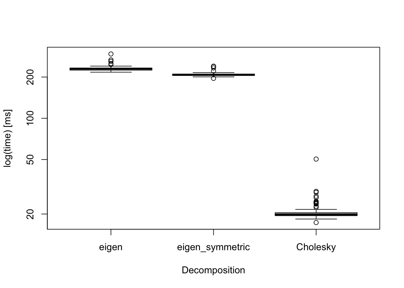
The boxplot above displays computation times for various decomposition methods for a banded covariance matrix when \(p=\) 1000:

1. base::eigen(),
2. base::eigen(symmetric=TRUE),
3. base::chol().

The result shows that Cholesky decomposition is the fastest. Thus, if we are 100% sure that the covariance matrix is positive-definite, then we use Cholesky decomposition.

Besides, in simulation studies, we often use a pre-defined positive-definite matrix multiple times. Hence, we don’t need to repeat matrix decomposition on the same matrix over and over for each iteration. We just need to do it only once. Therefore, we can save lots of seconds if we use decomposed matrix as an input of the random sample generating function.

The following code is a personally used functions for generating multivariate normal samples, which is a modified version of code from Prof. Karl Broman (https://github.com/kbroman/broman) to use the output of chol() as an input variable.

# Modification of the code from Prof. Karl Broman (https://github.com/kbroman/broman)
rmvn <- function(n, mu = 0, Sigma = NA, chol.mat = NA) {
    if(any(is.na(Sigma)) & any(is.na(chol.mat))){
      stop("Must Input one of Sigma or chol.mat")
    }
    
    p <- length(mu)
    if (any(is.na(match(dim(Sigma), p)))) {
      stop("Dimension problem!")
    }
    if(any(is.na(chol.mat))){
      D <- chol(Sigma)
    }else{
      D <- chol.mat
    }
    
    matrix(rnorm(n * p), ncol = p) %*% D + rep(mu, rep(n, p))
  }

Numerical study: speed comparison

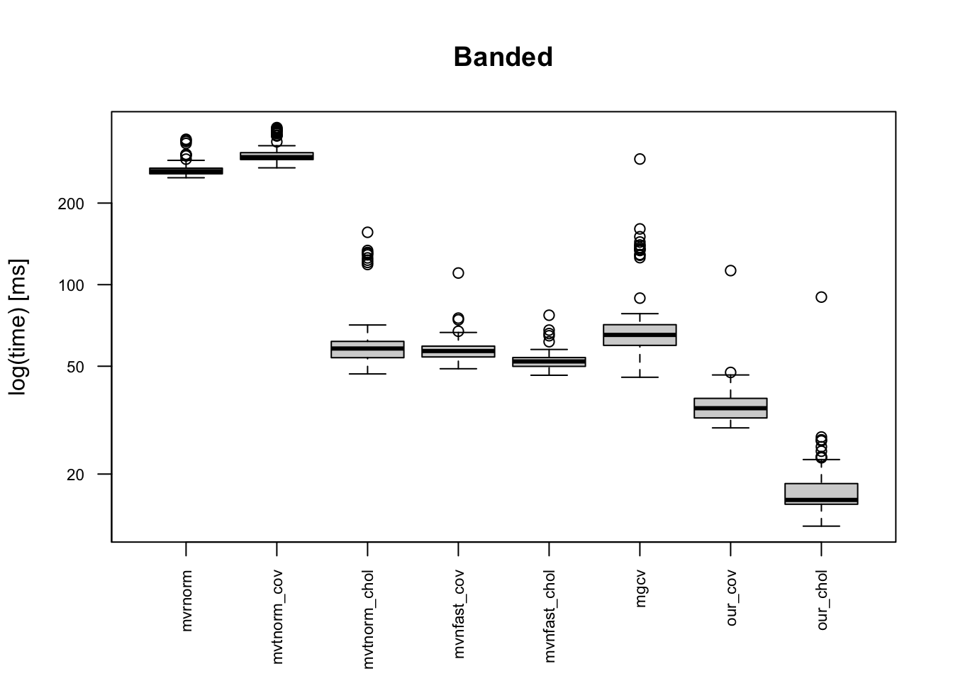
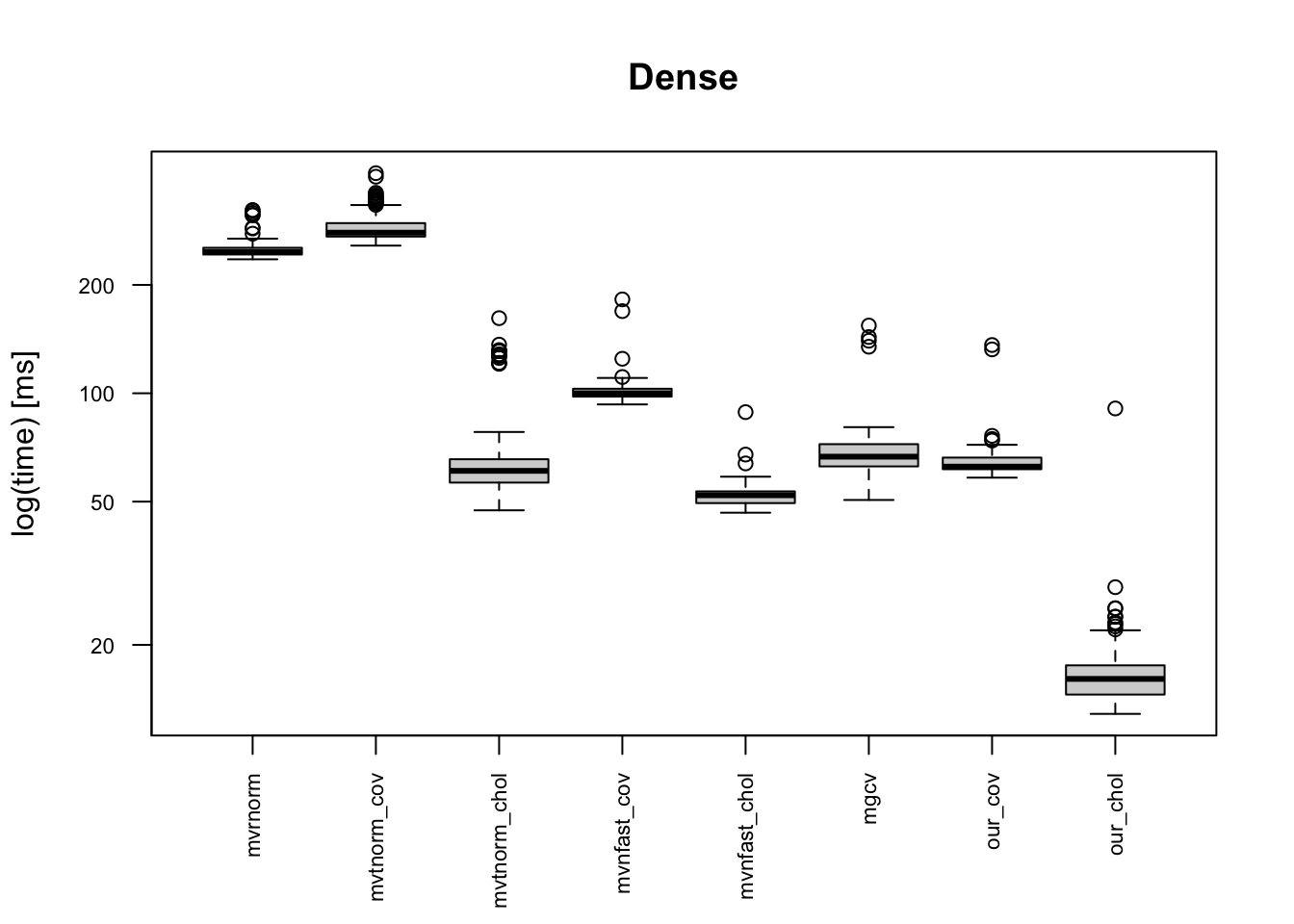
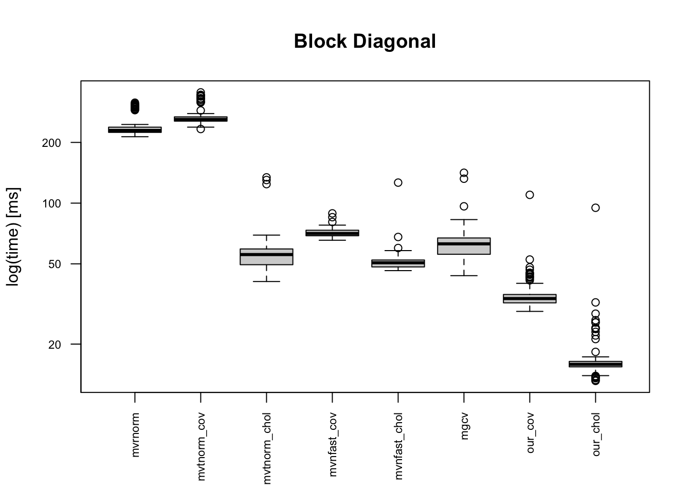
We compare various data generating functions when \(n=\) 100 and \(p=\) 1000 :

1. Eigen: MASS::mvrnorm(), eigendecomposition,
2. mvtnorm_eigen: mvtnorm::rmvnorm(), eigendecomposition,
3. mvtnorm_chol: mvtnorm::rmvnorm(), Cholesky decomposition,
4. mvnfast_cov: mvnfast::rmvn() with a covariance matrix,
5. mvnfast_chol: mvnfast::rmvn() with a Cholesky-decomposed matrix as an input,
6. mgcv: mgcv::rmvn(): Cholesky decomposition by chol() with error handling,
7. our_cov: Our code with a covariance matrix,
8. our_chol: Our code with a Cholesky-decomposed matrix as an input.

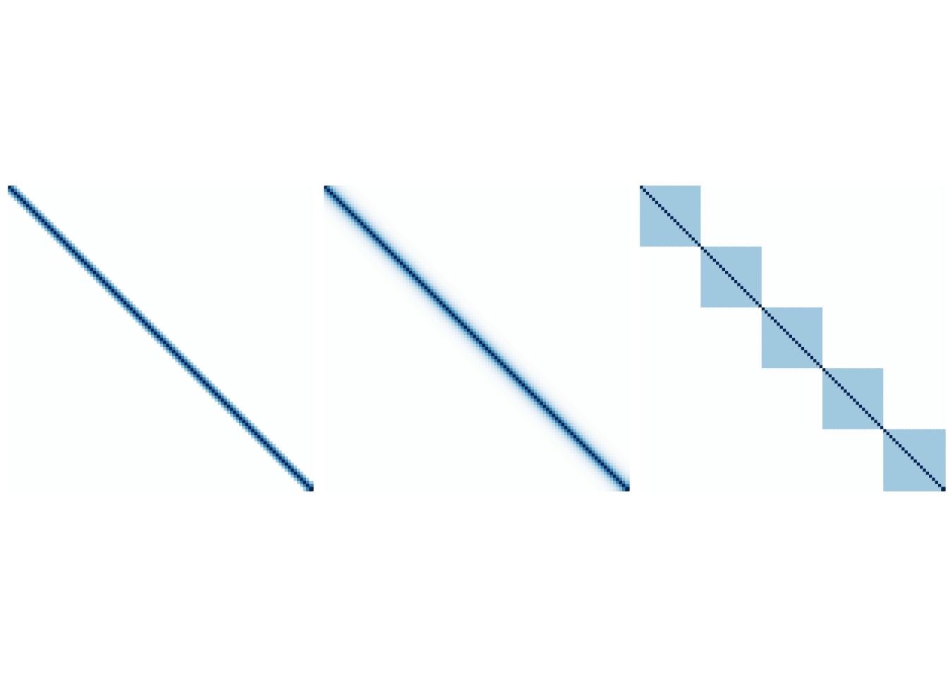
We consider three dependence structures:

1. Banded: \[ \sigma_{j,k} = \begin{cases} 1 & j=k\\ 0.6 & |j-k|=1\\ 0.3 & |j-k|=2\\ 0 & |j-k|\geq 3 \end{cases}, \]
2. Dense: \(\sigma_{j,k}=0.6^{|j-k|}\),
3. Block diagonal: \(\Sigma = diag(B_1,\ldots, B_{5})\) where \(B_i\) for \(i=1,\ldots, 5\) have 1 as the diagonal entries and 0.3 as the off-diagonal entries.

The following figures are the graphical illustration of the structures.

The boxplots below indicates that the provided code is the fastest, and it is 10+ times faster than mvrnorm(). Moreover, our code is faster than “faster” multivariate normal generating functions. This is because of one simple reason: simplicity of the code. Other built-in functions in CRAN package do error handling for erroneous inputs, and they works for semi-positive definite matrix. Meanwhile, our code can be applicable only for a positive-definite covariance matrix.

Revisit: data generation by our code as dimension increases

## Unit: milliseconds
##  expr       min          lq        mean      median          uq        max
##   100  0.580252   0.6783475   0.7194807   0.7181015   0.7483635   1.063139
##   200  1.258586   1.4892190   1.5555297   1.5495590   1.6435650   1.935576
##   400  3.114879   3.7150305   4.1526607   3.8323960   4.0705575  28.856649
##   800  8.721678  10.2668570  11.7867619  10.8417830  11.2993685  35.662729
##  1600 28.907703  34.8350660  38.5244416  35.8951730  37.3108075  64.493195
##  3200 98.807819 121.0690605 127.3867776 125.7567810 133.4152565 205.078114
##  neval
##    100
##    100
##    100
##    100
##    100
##    100

Let’s check the performance of our code by various \(p\). Using a Cholesky-decomposed matrix as an input, the computation time increases around 4 times as \(p\) doubles. Moreover, we observe computation speed is much faster than MASS::mvrnorm(). This tendency is more evident when \(p\) is larger. By using a Cholesky-decomposed matrix, it would take \(0.036 \times 500 \times 3 = 54\) seconds when \(n=100\) and \(p=1600\) with 3 settings and \(500\) repetitions per each setting.

Discussion

We checked the structure of MASS::mvrnorm() and discussed how to generate multivariate normal samples faster. When the covariance matrix is positive-definite, we have significant speed improvement on the computation speed by using its Cholesky decomposition. The presented code requires users’ carefulness since it does not check erroneous inputs such as non-invertible matrix, non-symmetric covariance matrix, and so on.

We can employ this idea on generating samples from an elliptical distribution. For example, we can sample from a multivariate-t distribution \(t_{df}(\Sigma)\) when the scale matrix \(\Sigma\) is positive-definite.

SessionInfo

## R version 4.1.1 (2021-08-10)
## Platform: x86_64-apple-darwin17.0 (64-bit)
## Running under: macOS Big Sur 10.16
## 
## Matrix products: default
## LAPACK: /Library/Frameworks/R.framework/Versions/4.1/Resources/lib/libRlapack.dylib
## 
## locale:
## [1] en_US.UTF-8/en_US.UTF-8/en_US.UTF-8/C/en_US.UTF-8/en_US.UTF-8
## 
## attached base packages:
## [1] stats     graphics  grDevices utils     datasets  methods   base     
## 
## other attached packages:
## [1] corrplot_0.90        microbenchmark_1.4-7 MASS_7.3-54         
## 
## loaded via a namespace (and not attached):
##  [1] knitr_1.34      magrittr_2.0.1  lattice_0.20-45 R6_2.5.1       
##  [5] rlang_0.4.11    fastmap_1.1.0   stringr_1.4.0   highr_0.9      
##  [9] tools_4.1.1     grid_4.1.1      xfun_0.26       jquerylib_0.1.4
## [13] htmltools_0.5.2 yaml_2.2.1      digest_0.6.28   bookdown_0.24  
## [17] Matrix_1.3-4    sass_0.4.0      evaluate_0.14   rmarkdown_2.11 
## [21] blogdown_1.5    stringi_1.7.4   compiler_4.1.1  bslib_0.3.0    
## [25] jsonlite_1.7.2